Modal Modelling

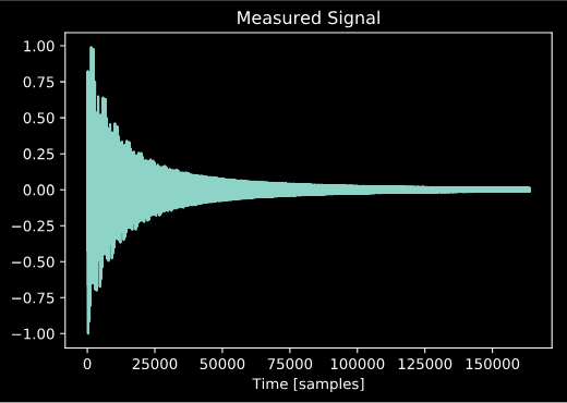
In this tutorial, we will show how to use audio_dsp to generate a modal model of a measured signal. To begin, we will examine a test signal recorded from a carrilon bell.

import numpy as np
import matplotlib.pyplot as plt
import audio_dspy as adsp

plt.figure()
plt.plot(x)
plt.title('Measured Signal')
plt.xlabel('Time [samples]')

plt.figure()
X = adsp.normalize(np.fft.rfft(x))
f = np.linspace (0, _fs_/2, num=len(X))
plt.semilogx(f, 20 *  np.log10 (np.abs(X)))
plt.xlim(20, 20000)
plt.title('Measured Signal DFT')
plt.xlabel('Frequency [Hz]')
plt.ylabel('Magnitude [dB]')

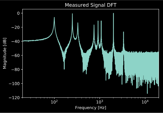
We know this signal is a good candidate for modal modelling, since the resonant frequencies don’t appear to be harmonically related. If they were, a different approach, such as additive synthesis might be a better choice. We could simply construct an impulse response model of the bell, but as we can see our measurement is quite noisy, which would make our IR model noisy as well.

Finding the Mode Frequencies

We can use adsp.find_freqs() to find the mode frequencies.

freqs, peaks = adsp.find_freqs(sig, _fs_, above=80, plot=True)
plt.xlim(20, 20000)

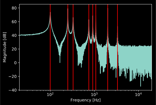
Note that the parameters used for this function depend greatly on the signal being analyzed, and you may need to fine tune them to achieve best results.

Finding the Mode Decay Rates

We can now find the decay rates of the modes using adsp.find_decay_rates().

taus = adsp.find_decay_rates(freqs, sig[:int(_fs_*1.5)], _fs_, 30, thresh=-10, plot=True)

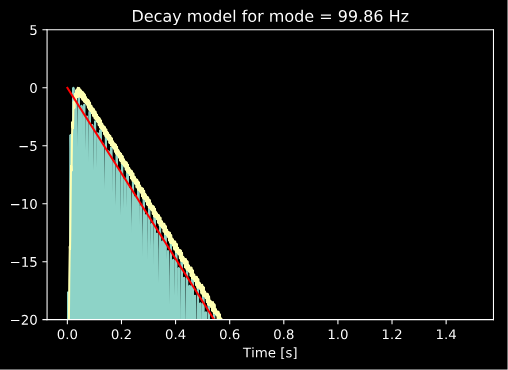
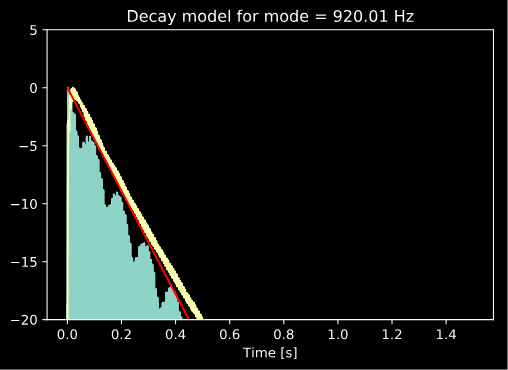
Note that if the plot flag is set, the function will produce a decay model plot for every mode, though we only choose to show two of them here in this tutorial. Also note that, again, the optimal parameters of the function will vary greatly depending on the data being analyzed.

Finding the Mode Amplitudes

If you like, you can simply use the peaks generated by the adsp.find_freqs() function as the amplitudes of your modal model. However, doing this ignores the phase variations that the different modes may have, as well as other spectral characteristics perhaps not captured by the modes. To create a more accurate model, we can use least squares optimization to find the optimal amplitude and phase of each mode with the adsp.find_complex_amplitudes() function.

amps = adsp.find_complex_amplitudes (freqs, taus, _N_, sig, _fs_)

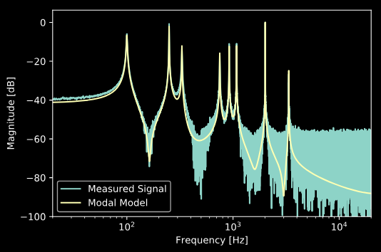
And finally, we can use adsp.generate_modal_signal() to generate our modal model, and compare with the measured signal:

y = adsp.generate_modal_signal(amps, freqs, taus, len(amps), _N_, _fs_)

Y = adsp.normalize(np.fft.rfft (y))
plt.semilogx (f, 20 * np.log10 (np.abs (X)))
plt.semilogx (f, 20 * np.log10 (np.abs (Y)))
plt.xlim(20, 20000)
plt.ylim(-100)
plt.legend(['Measured Signal', 'Modal Model'])
plt.xlabel('Frequency [Hz]')
plt.ylabel('Magnitude [dB]')

References

[1]	K.J. Werner, E.K. Canfield-Dafilou “Modal Audio Effects: A Carollon Case Study”, Proc. of the 20th International Conference on Digital Audio Effects (DAFx-17), Edinburgh, UK, Sept. 5-9, 2017