Nonlinear Processing

audio_dspy currently supports three simple nonlinear processors (hard-clipping, soft-clipping, and dropout nonlinearities), as well as useful plotting functions for visualizing the properties of a nonlinear system.

Processing Audio

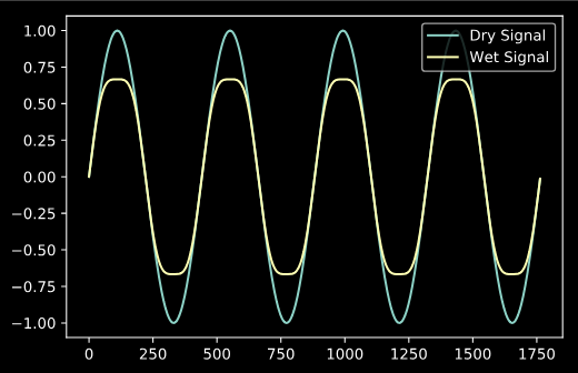
Processing a block of audio with a nonlinear processor can be done as follows:

import numpy as np
import matplotlib.pyplot as plt
import audio_dspy as adsp

fs = 44100
N = 441*4
freq = 100
x = 1.0 * np.sin(2 * np.pi * np.arange(N) * freq / fs)
y = adsp.soft_clipper(x)

plt.plot(x)
plt.plot(y)
plt.legend(['Dry Signal', 'Wet Signal'])

Visualizing Nonlinear Functions

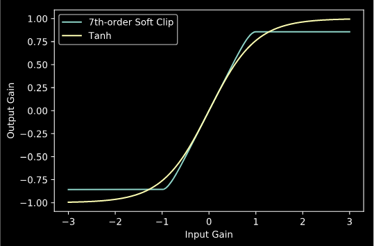
To visualize a nonlinear function, you can pass a lambda of the function into adsp.plot_static_curve(), or for nonlinear functions with more dynamic responses, adsp.plot_dynamic_curve().

import numpy as np
import matplotlib.pyplot as plt
import audio_dspy as adsp

adsp.plot_static_curve(lambda x :  adsp.soft_clipper(x, deg=7), gain=3)
adsp.plot_static_curve(lambda x :  np.tanh(x), gain=3)
plt.legend (['7th-order Soft Clip', 'Tanh'])

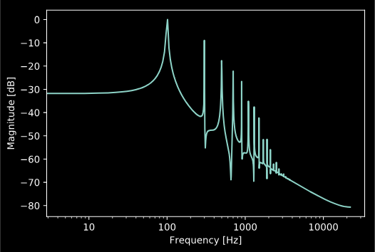
We can also plot the harmonic response of a nonlinear function with adsp.plot_harmonic_response().

adsp.plot_harmonic_response(lambda x : np.tanh(x), gain=5