EQ Filter Design
Basic Filter Design
audio_dspy currently contains simple filter design functions
for 6 common EQ shapes:
- Lowpass (1st-order, 2nd-order, Nth-order)
- Highpass (1st-order, 2nd-order, Nth-order)
- Lowshelf
- Highshelf
- Bell
- Notch
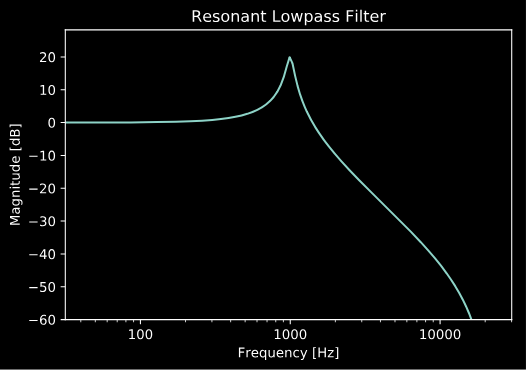
As an example, we’ll use these functions to design a resonant 2nd-order lowpass filter.
import audio_dspy as adsp
fs = 44100 # set sample rate
b, a = adsp.design_LPF2(1000, 10, fs)
adsp.plot_magnitude_response(b, a, fs=fs)

# plot settings
import matplotlib.pyplot as plt
plt.title('Resonant Lowpass Filter')
plt.ylim(-60)
plt.show()
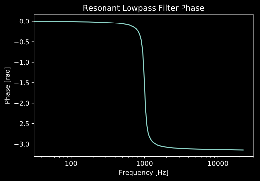
We can also easily view the phase response of the filter:
adsp.plot_phase_response(b, a, fs=fs)
plt.title('Resonant Lowpass Filter Phase')
plt.show()
Processing Audio with Filters
The filter coefficients returned by the filter design functions can then be
used to filter data. The simplest way to do this is to use the scipy function
scipy.signal.lfilter(), however if you prefer a little more
functionality, you can use the adsp.Filter object.
As an example, let us design a lowpass filter, to filter a white noise signal.
# generate white noise signal
import numpy as np
N = 1024
x = np.random.rand(N) * 2 - 1 # range: (-1, 1)

# Design filter
import audio_dspy as adsp
fs = 44100
b, a = adsp.design_LPF2(1000, 0.707, fs)

# Setup filter
filter = adsp.Filter(2, fs)
filter.set_coefs(b, a)

# Process audio
filter.reset()
y = filter.process_block(x)
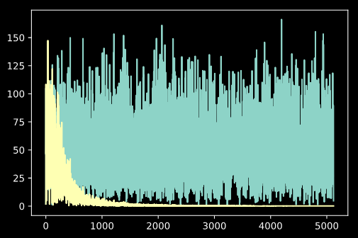
Now we can examine the fft of the input and output signals, and see the effects of the filtering:
plt.plot(np.abs(np.fft.rfft(x)))
plt.plot(np.abs(np.fft.rfft(y)))
plt.show()
Be sure to call Filter.reset() in between filtering independent streams
of data to clear the state of the filter.
Designing and Using an EQ
For more advanced filtering needs, we can use the adsp.EQ object.
This object allows us to filter a signal with a whole set of filters.
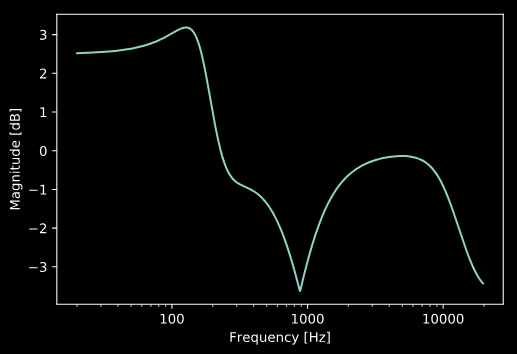
In the example below, we design an EQ with a low shelf filter, a lowpass filter, and a notch filter.
import audio_dspy as adsp
import numpy as np
import matplotlib.pyplot as plt

fs = 44100 # sample rate
worN = np.logspace(1, 3.3, num=1000, base=20) # frequencies to plot

# design EQ
eq = adsp.EQ(fs)
eq.add_LPF(10000, 0.707)
eq.add_lowshelf(200, 1.4, 2)
eq.add_notch(880, 0.707)

# plot EQ magnitude response
eq.plot_eq_curve(worN=worN)
plt.show()
Note that you can process audio with the EQ object, just like the Filter object
using adsp.EQ.process_block() and adsp.EQ.reset().